
চিত্র:Lens and wavefronts.gif
এর চেয়ে বেশি রেজোলিউশন লভ্য নয়।
Lens_and_wavefronts.gif (১৮৩ × ৩৫৬ পিক্সেল, ফাইলের আকার: ৩৫ কিলোবাইট, এমআইএমই ধরন: image/gif, লুপকৃত, ৯ ফ্রেম, ০.৭ সে)
| এই ফাইলটি উইকিমিডিয়া কমন্স থেকে নেওয়া। সেখানের বর্ণনা পাতার বিস্তারিত নিম্নে দেখানো হলো। (সম্পাদনা)
|
slnglelens
সারাংশ
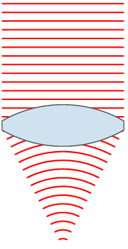
| বিবরণ | Illustration of wavefronts after passing through a lens. Interestingly, to produce a point source reverse the direction of the waves, with the focus point acting as a point source. |
| তারিখ | (UTC) |
| উৎস | self-made with MATLAB |
| লেখক | Oleg Alexandrov |
| অন্যান্য সংস্করণ |
 |
এই ডায়াগ্রামটি MATLAB দিয়ে তৈরি করা হয়েছে।
লাইসেন্স প্রদান
| আমি, এই কাজের স্বত্বাধিকারী, এতদ্দ্বারা আমি এই কাজকে পাবলিক ডোমেইন লাইসেন্সের আওতায় প্রকাশ করলাম। এটি বিশ্বব্যাপী প্রযোজ্য হবে। কিছু দেশে এটি আইনত সিদ্ধ নাও হতে পারে, যদি তাই হয়: আমি যে-কাউকে এই কাজটি যেকোনো উদ্দেশ্যে, বিনাশর্তে ব্যবহারের অনুমতি প্রদান করছি, যদি না সেই শর্তগুলো আইনত প্রয়োজনীয় হয়। |
siingleline
% Illustration of planar wavefronts going through a lens and getting focused
% into a converging spherical wave

function main ()

  % lens index
   n=1.5;

  % number of points, used for plotting
   N = 100;

  % radii of lens surfaces
   R1 = 0.5;
   R2 = 1.5;

  % centers of circles (y coord is 0)
   O1 = -2.9;
   O2 = -O1;

  % focal length
   f = (n-1)*(1/R1+1/R2); f = 1/f;

   % theta0 determines the width of the lens
   theta0=pi/6;
   Theta = linspace(-theta0, theta0, N);

  % right face of the lens
   L1x = R1*cos(Theta)+O1;
   L1y =R1*sin(Theta);

   % left size of the lens
   L2x=-R2*cos(Theta)+O2;
   L2y = R2*sin(Theta);

   % flat top part
   Topx = [L1x(N), L2x(N)];
   Topy = [L1y(N), L2y(N)];

   % flat bottom part
   Botx = [L1x(1) L2x(1)];
   Boty = [L1y(1), L2y(1)];

   % the lens
   Lensx = [L1x rv_vec(Topx), rv_vec(L2x), Botx];
   Lensy = [L1y rv_vec(Topy), rv_vec(L2y), Boty];

   % Parameters for graphing
   Lens_color  = [204, 226, 239]/256;
   Lens_border = 0.3*[1, 1, 1];
   lbw = 1.3; % lens border width
   wavefr_color = [1, 0, 0];
   wavefr_bdw   = 2;

   % spacing between wavefronts (both plane and spherical ones)
   spacing = 0.25;

   % 2*H is the height of the plane wavefronts
   H = L1y(N);

   % theta2 = slope of the line going from the upper-right
   % end of the lens to the focus point
   theta2 = atan(L1y(N)/(f-L1x(N)));

   % Shape of the spherical wavefronts.
   Theta = linspace(-theta2, theta2, N);
   X = -cos(Theta);
   Y =  sin(Theta);

   S = -f; % start ploting waves from here to the right

   % number of frames in the movie
   num_frames = 10;
   Shifts = linspace(0, spacing, num_frames+1);

   % start at S+shift, plot the wavefronts
   for frame_no = 1:num_frames

      shift = Shifts(frame_no);

      s = S+shift;

      % plotting window
      figure(1); clf; hold on; axis equal; axis off;

      % plot the plane wavefronts
      while s < 0
         plot([s, s], [-H, H], 'color', wavefr_color, 'linewidth', wavefr_bdw);
         s = s + spacing;
      end


      % plot the spherical wavefronts
      s = s - 10*spacing; % backtrack a bit
      while s < f

         rho = f-s;

         if rho*Y(N) <= L1y(N)
            plot(rho*X+f, rho*Y, 'color', wavefr_color, 'linewidth', wavefr_bdw);
         end

         s = s + spacing;

      end

      % plot the lens
      fill(Lensx, Lensy, Lens_color, 'EdgeColor', Lens_border, 'LineWidth', lbw);
%      get(H)
%      return

      % Invisible points to force MATLAB to keep the
      % plotting window fixed.
      tiny = 0.15*spacing;
      white = 0.999*[1, 1, 1];
      plot(S-tiny,   H+tiny, 'color', white);
      plot(S-tiny,  -H-tiny, 'color', white);
      plot(f+tiny,   H+tiny, 'color', white);
      plot(f+tiny,  -H-tiny, 'color', white);

      % Rotate by 90 degrees
      set(gca, 'View', [90, 90])

      % save current file
      frame_file = sprintf('Frame%d.eps', 1000+frame_no);
      disp(frame_file);
      saveas(gcf, frame_file, 'psc2');
      pause(0.07)
   end

% The frames were converted to a movie with the command
% convert -antialias -loop 10000  -delay 8 -compress LZW Frame100* Lens_and_wavefronts.gif

function W = rv_vec(V)

   K = length(V);

   W = V;
   for i=1:K
      W(i) = V(K-i+1);
   end
ফাইলের ইতিহাস
যেকোনো তারিখ/সময়ে ক্লিক করে দেখুন ফাইলটি তখন কী অবস্থায় ছিল।
| তারিখ/সময় | সংক্ষেপচিত্র | মাত্রা | ব্যবহারকারী | মন্তব্য | |
|---|---|---|---|---|---|
| বর্তমান | ০৬:৩৫, ২৫ নভেম্বর ২০০৭ | | ১৮৩ × ৩৫৬ (৩৫ কিলোবাইট) | Oleg Alexandrov | tweak |
| ০৪:১০, ২৪ নভেম্বর ২০০৭ |  | ১৭১ × ৩৫৬ (৩৩ কিলোবাইট) | Oleg Alexandrov | tweak | |
| ০৪:০৯, ২৪ নভেম্বর ২০০৭ |  | ১৭১ × ৩৫৬ (৩৩ কিলোবাইট) | Oleg Alexandrov | tweak | |
| ০০:৫৬, ২৪ নভেম্বর ২০০৭ |  | ১৭১ × ৩৫৯ (৩৩ কিলোবাইট) | Oleg Alexandrov | tweak, same license | |
| ০০:৫৩, ২৪ নভেম্বর ২০০৭ |  | ১৭১ × ৩৫৯ (৩২ কিলোবাইট) | Oleg Alexandrov | tweak | |
| ০০:৪৯, ২৪ নভেম্বর ২০০৭ |  | ১৫১ × ৩৫৯ (৩১ কিলোবাইট) | Oleg Alexandrov | {{Information |Description=Illustration of wavefronts after passing through a [:en:lens (optics)|lens]] |Source=self-made with MATLAB |Date=~~~~~ |Author= Oleg Alexandrov |Permission=see below |other_versions= }} |
সংযোগসমূহ
ফাইলের বৈশ্বিক ব্যবহার
নিচের অন্যান্য উইকিগুলো এই ফাইলটি ব্যবহার করে:
- ar.wikipedia.org-এ ব্যবহার
- ast.wikipedia.org-এ ব্যবহার
- be.wikipedia.org-এ ব্যবহার
- bs.wikipedia.org-এ ব্যবহার
- ckb.wikipedia.org-এ ব্যবহার
- cs.wikiversity.org-এ ব্যবহার
- cv.wikipedia.org-এ ব্যবহার
- en.wikipedia.org-এ ব্যবহার
- en.wikiversity.org-এ ব্যবহার
- es.wikipedia.org-এ ব্যবহার
- es.wikiversity.org-এ ব্যবহার
- eu.wikipedia.org-এ ব্যবহার
- fa.wikipedia.org-এ ব্যবহার
- fi.wikipedia.org-এ ব্যবহার
- fr.wikipedia.org-এ ব্যবহার
- fr.wikibooks.org-এ ব্যবহার
- fy.wikipedia.org-এ ব্যবহার
- ga.wikipedia.org-এ ব্যবহার
- he.wikipedia.org-এ ব্যবহার
- hi.wikipedia.org-এ ব্যবহার
- hr.wikipedia.org-এ ব্যবহার
- hy.wikipedia.org-এ ব্যবহার
- id.wikipedia.org-এ ব্যবহার
- lt.wikipedia.org-এ ব্যবহার
- lv.wikipedia.org-এ ব্যবহার
- ml.wikipedia.org-এ ব্যবহার
- mn.wikipedia.org-এ ব্যবহার
- nl.wikipedia.org-এ ব্যবহার
- pa.wikipedia.org-এ ব্যবহার
- ru.wikipedia.org-এ ব্যবহার
- sh.wikipedia.org-এ ব্যবহার
- si.wikipedia.org-এ ব্যবহার
- sl.wikipedia.org-এ ব্যবহার
- sr.wikipedia.org-এ ব্যবহার
- sv.wikipedia.org-এ ব্যবহার
- ta.wikipedia.org-এ ব্যবহার
- te.wikipedia.org-এ ব্যবহার
এই ফাইলের অন্যান্য বৈশ্বিক ব্যবহার দেখুন।